Rohin Gosling · · Read on Medium
How a small, transparent heuristic can sometimes be more useful than a complicated model.
I was speaking with a collections team that needed a simple way to prioritize indebted users based on temporal repayment behavior. They were looking for something simple that could be used as a formula in a spreadsheet. So no machine-learning models or any other kind of infrastructure or resource-intensive methods. Just a scalar signal that could help prioritize workloads and be easy to understand and implement in a spreadsheet. The goal was not to estimate probability of default, automate lending decisions, or replace any existing credit-scoring systems. It just needed to prioritize repayment behavior using a time-sensitive behavioral heuristic.
Here is a method that I think does this well.
The central idea encodes the narrow assumption that more recent repayment activity is a stronger positive operational signal than otherwise identical older repayment activity.
- Higher score: stronger recent repayment activity.
- Lower score: weaker recent repayment activity.
This can be achieved through the application of an exponentially biased debt repayment weight, configured such that when debt amount, total repayments, observation window, and other parameters are held constant:
- Repayments concentrated in recent periods produce a higher score.
- Repayments concentrated in older periods produce a lower score.
- No recent repayments cause the positive signal from older repayments to fade over time.
Note:
- The exponentially biased weight function does not determine “why” repayment activity changed. For example, a lower score could reflect hardship, a dispute, payment timing, data problems, or reduced opportunity to repay. It also measures both amount and recency, so a sufficiently large older repayment can outweigh a small recent one.
- The technical note for this article may be found here.
Exponentially Biased Debt Repayment Weight: A Lightweight, Interpretable Repayment Ranking Heuristic. Rohin Gosling, 2025 .
The problem with repayment totals
Imagine two users who have each repaid 350 over the last six weeks.
If you rank them using only the total amount repaid, they look identical. But suppose one user made most of those repayments in the last two weeks, while the other made most of them five or six weeks ago. Operationally, those histories may not feel identical at all.
The first suggests recent activity. The second suggests activity that has cooled off.
This does not prove that one person is safer, more willing, or more able to repay. Timing alone cannot answer those questions. But when a team has limited attention and needs a transparent prioritization signal, the timing of repayment can still be useful information.
Raw totals discard that information. A hard lookback window preserves some of it, but creates a cliff: a repayment just inside the window counts fully, while one just outside counts nothing. A recency-weighted total offers a middle path. Recent periods matter most, and older periods fade gradually.
That is where exponential decay becomes useful.
Think of a dimmer switch, not an on/off cutoff
The intuition comes before the formula.
Start with the most recent repayment period — a day, week, month, or another fixed interval. Give it full weight. Give the preceding period slightly less weight. Give the period before that less again, and continue in the same way.
Older repayments are not suddenly erased. Their influence is turned down progressively, like a dimmer switch.
Exponential decay is well suited to this job because it gives us a smooth, predictable decline controlled by a single parameter. If we want recent behavior to dominate quickly, we choose a fast decay. If we want older history to remain influential for longer, we choose a slower decay.
There is no hidden model fitting and no opaque feature importance. The curve is the policy choice.
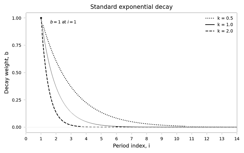
Figure 1. Standard exponential decay curves for k = 0.5, k = 1.0, and k = 2.0. Each curve equals 1 at period index i = 1 and approaches zero asymptotically as i increases. Source: “Exponentially Biased Debt Repayment Weight,” Figure 1.
Turning that intuition into a score
Let the observation window contain n ∈ ℕ fixed repayment periods, indexed by

The index runs backward from the ranking date: i = 1 is the most recent period, i = 2 is the immediately preceding period, and i = n is the oldest period included in the window. Every user in the same ranking run should use the same bucket definition and the same value of n.
For the basic non-negative repayment formulation, define:
- Pᵢ — Domain: Pᵢ ∈ ℝ ≥ 0; Meaning: Repayment amount posted during period i
- L — Domain: L ∈ ℝ > 0; Meaning: Fixed reference debt amount used as the denominator
- dᵢ — Domain: dᵢ ∈ ℝ ≥ 0; Meaning: Repayment in period i, normalized by L
- k — Domain: k ∈ ℝ > 0; Meaning: Decay-rate constant
- bᵢ — Domain: bᵢ ∈ ℝ ≥ 0; Meaning: Recency-weighted repayment contribution
- w — Domain: w ∈ ℝ ≥ 0; Meaning: Composite repayment-ranking score
Negative repayments, refunds, and reversals require a separate accounting policy; they are not silently absorbed into the basic domain above.
The normalized repayment is

Because Pᵢ and L use the same currency unit, dᵢ is dimensionless. The reference amount L might be the outstanding balance at the start of the observation window or the total scheduled amount for the account. The choice is a policy decision, but the rule for choosing L must be consistent across the users being compared.
The paper defines the Standard exponential bias weight as

To make the function’s arguments explicit in this article, write the same weight as

The offset i−1 gives the function three useful properties:

Thus the most recent period has full weight, every finite older period has a positive but smaller weight, and the weights approach zero asymptotically.
The paper’s recency-weighted repayment contribution is

The composite score across the observation window is

The score w is dimensionless and non-negative under the stated domain. Unless normalized repayments are capped or an additional normalization is introduced, w is not restricted to the interval [0, 1]. That is another reason it must not be interpreted as a probability.
A larger w means stronger recent repayment activity relative to the selected reference debt amount, observation window, and decay rate. It does not mean that the user has a particular probability of repayment, is creditworthy, or presents low risk.
A complete worked example
Use the same parameters and repayment sequence as the technical note:

The vector is ordered from newest to oldest, so P₁ = 120 is the most recent repayment and P₆ = 100 is the oldest.
For each period,

Using four decimal places in the table avoids obscuring the final total through premature rounding:
- 1 — Repayment Pᵢ: 120; Normalized dᵢ: 0.120; Weight exp(−0.35(i−1)): 1.0000; Contribution bᵢ: 0.1200
- 2 — Repayment Pᵢ: 80; Normalized dᵢ: 0.080; Weight exp(−0.35(i−1)): 0.7047; Contribution bᵢ: 0.0564
- 3 — Repayment Pᵢ: 0; Normalized dᵢ: 0.000; Weight exp(−0.35(i−1)): 0.4966; Contribution bᵢ: 0.0000
- 4 — Repayment Pᵢ: 50; Normalized dᵢ: 0.050; Weight exp(−0.35(i−1)): 0.3499; Contribution bᵢ: 0.0175
- 5 — Repayment Pᵢ: 0; Normalized dᵢ: 0.000; Weight exp(−0.35(i−1)): 0.2466; Contribution bᵢ: 0.0000
- 6 — Repayment Pᵢ: 100; Normalized dᵢ: 0.100; Weight exp(−0.35(i−1)): 0.1738; Contribution bᵢ: 0.0174
Evaluating the sum with unrounded values gives

Note what happens to the two repayments of similar size. The repayment of 120 in the most recent week contributes 0.1200. The repayment of 100 in the oldest week contributes only about 0.0174. The older repayment still counts, but it counts much less.
Now compare two users with repayment vectors

and

Their unweighted repayment totals are equal:

With the same L = 1000 and k = 0.35, however,
- A — Repayments, newest to oldest: 180, 120, 0, 0, 0, 50; Total repaid: 350; Score w: 0.273
- B — Repayments, newest to oldest: 50, 0, 0, 0, 120, 180; Total repaid: 350; Score w: 0.111
A total-only measure treats the users as equal. The exponential score ranks User A higher because more of the repayment mass occurs at smaller values of i, where exp(−k(i−1)) is larger.
That statement is mathematical, not moral. It says nothing by itself about either user’s character, affordability, or eventual outcome.
Half-life makes the decay easier to explain
The raw decay constant k is mathematically convenient but not especially intuitive. Half-life gives the same parameter a direct temporal interpretation.
Let h > 0 be the number of period steps from the most recent bucket at which the Standard bias weight falls to one half. Because the most recent bucket is i = 1, this condition is

Taking natural logarithms gives

and therefore

- 1 period — Decay constant k = ln(2)/h: 0.693; Interpretation: Very strong recency bias
- 2 periods — Decay constant k = ln(2)/h: 0.347; Interpretation: Strong recency bias
- 4 periods — Decay constant k = ln(2)/h: 0.173; Interpretation: Moderate recency bias
- 8 periods — Decay constant k = ln(2)/h: 0.087; Interpretation: Gentle recency bias
With a two-week half-life, for example, the bucket two weekly steps behind the most recent bucket has index i = 3 and weight ½. With an eight-week half-life, the score retains much more historical memory.
There is no universally correct half-life. The choice expresses how quickly the relevance of past repayment behavior is assumed to fade for a particular workflow. It should be tested by comparing plausible values, examining ranking sensitivity, and validating the result against the actual operational objective.
while b(1; k) = 1 for all k > 0. Large k therefore makes the newest period dominate.
Standard decay versus a hard historical cutoff
The Standard weight is strictly positive for every finite i:

It approaches zero but never reaches it. For many uses, that smooth fading of historical influence is desirable.
Other workflows require a firm historical boundary. The paper’s Extended decay-to-zero form preserves an exponential shape on the active interval while satisfying the boundary conditions

where n > 1 is the cutoff and k > 0 is the decay rate.
Define the boundary-condition coefficients

and

The complete finite-window function is

Here x is a continuous plotting variable. Discrete repayment buckets use integer values x = i. Substitution verifies the endpoints of the active exponential segment:

and

The piecewise definition therefore satisfies

Equivalently, substituting the coefficients gives the active segment in full:

Applying this weight to discrete repayment buckets gives the Extended composite score

Because y(n; k, n) = 0, repayment at the cutoff contributes zero, as does any repayment beyond it.
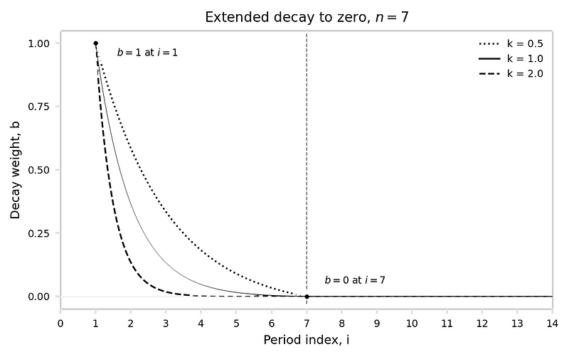
Figure 2. Extended decay-to-zero curves for k = 0.5, k = 1.0, and k = 2.0, with cutoff n = 7. Each curve equals 1 at x = 1, reaches exactly 0 at x = n = 7, and remains zero thereafter. Source: “Exponentially Biased Debt Repayment Weight,” Figure 2.
The distinction between the methods is now exact:
- Standard — Mathematical support: b(i; k) > 0 for every finite i; Treatment of old history: Influence declines asymptotically toward zero
- Extended — Mathematical support: y(x; k, n) = 0 for x ≥ n; Treatment of old history: Influence ends exactly at the selected cutoff
The Extended form is not automatically better. Although the function itself reaches zero continuously at x = n, the cutoff is a firm policy boundary: history at or beyond n has no influence. That may be appropriate, but it should be intentional.
The technical note contains the same definitions and derivation in their formal publication context.
The implementation details matter more than the algebra suggests
The formulas are short. A reliable implementation still requires several explicit decisions.
Use fixed, consistent buckets. If the period is one week, every user in the ranking run should be evaluated in weekly buckets with the same boundary rule. Irregular repayment dates should be aggregated into those buckets before the score is calculated.
Record missing periods as zero. A week without a repayment should be represented as Pᵢ = 0, not omitted. Omitting it shortens the apparent time distance between payments and gives an inaccurate recency weight.
Use the same observation window. Comparing a six-week history with a twelve-week history can change the meaning of the raw score. The simplest rule is to use the same n for everyone in a ranking run.
Define the denominator once. The reference debt amount L shapes every normalized repayment. Opening balance, current outstanding balance, and scheduled amount are not interchangeable. Choose a defensible definition and apply it consistently.
Decide how to handle edge cases. A zero or negative denominator makes the score undefined. Refunds and payment reversals need an accounting policy. Overpayments require a choice about whether normalized repayments may exceed one or should be capped.
The calculation itself is lightweight and can be implemented in a spreadsheet, SQL query, or short script. And each user requires only one multiplication and addition per period. The important part is ensuring that the inputs mean the same thing for everyone being compared, which is primarily achieved by using consistent bucket boundaries, observation windows, reference debt amount for normalization, and edge case policies.
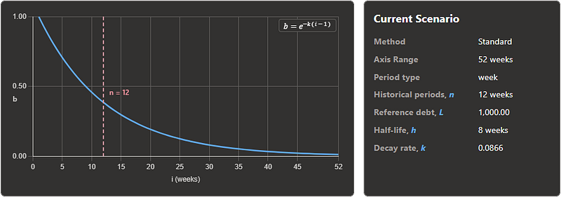
Try the curve interactively
The easiest way to develop intuition for the method is to move the controls and watch the curve change.
I built an interactive explorer where you can switch between the Standard and Extended methods, select a period type, adjust the historical range, choose a reference debt amount, and set the half-life. The curve and current-scenario readout update immediately.
The explorer visualizes the bias-weight curve. It does not accept a live debtor repayment sequence or calculate a production account score. Its purpose is simply to visualize the decay policy, either out of academic interest or as a design step before applying it to real data.
The full project, including the explorer and published documents, is available in the GitHub repository.
What this method does — and what it does not do
This method is a prioritization heuristic. It is not:
- A probability-of-default model;
- An affordability assessment;
- An expected-loss model;
- A hardship, fraud, dispute, or vulnerability detector;
- A validated credit score;
- A substitute for human review, governance, or compliance controls.
Instead, it summarizes a narrowly defined aspect of observed behavior: repayment amounts normalized against a chosen debt reference, with more influence assigned to recent periods.
The signal is easy to inspect and explain. It does not require demographic features, labeled outcomes, third-party behavioral data, or model training. In exploratory workflows, small portfolios, or environments with limited infrastructure, those properties may be valuable. The score is best treated as one input into a process, not the process itself.
A transparent judgment, expressed clearly
The value of the Exponentially Biased Debt Repayment Weight is not that it is complex. It is that the method is small enough to explain, easy enough to implement, and explicit about the judgment it encodes:
- Recent repayment behavior should count more than older repayment behavior.
Whether that judgment is useful depends on the workflow, the data, the parameter choices, and the safeguards around its use. When it is appropriate, exponential decay provides a clean way to express it — without pretending that a transparent ranking heuristic is a full credit-risk model.
Explore the project
- Try the interactive explorer
- Read the formal technical note
- View the GitHub repository
- For the sake of entertainment, see the original whiteboard sketch